Ramblemuse Touch Points

You can observe a lot by just watching. — Yogi Berra

As a physicist, I’m a strong believer in energy balances. If, over a prolonged period, you have more energy coming into a system than is going out from the system, then it’s a pretty sure bet that the system is storing energy. For a complex system, like the Earth, how that storage is implemented may vary, but that such storage implies change to the system seems a no brainer. Statistical detection of such change in a noisy system with a lot of internal variability is another matter.

Thinking about the Earth’s energy balance, about 240 W/m² is absorbed by the Earth on a yearly, global average at wavelengths shorter than 4 μm. Balance would imply that the same energy is emitted back to space and, given the Earth’s temperature, at infrared wavelengths longer than 4 μm. Absorption and emission occur in separable regions of the electromagnetic spectrum. Estimates from radiative transfer calculations are that doubling the concentration of carbon dioxide would reduce what’s emitted back to space by about 4 W/m², which is referred to as the climate forcing from doubling CO₂.

If the Earth is taking on more energy than it is emitting as infrared radiation, balance can be restored by an increase in the effective radiating temperature of the earth. In terms of a simple model, the radiation emitted by earth depends on the Stefan-Boltzmann equation, \(E = \sigma T^4_e\), the subscript ‘e’ on the temperature indicating that it is an effective radiating temperature. We could start from a pre-industrial assumption of having an energy balance:
$$\sigma T^4_e = \frac{1 – \alpha}{4} S_0,$$
where \(S_0\) is the energy flux from the sun, \(\alpha\) is the albedo of the Earth (fraction of sunlight reflected), and the factor of 1/4 accounts for both geometry and daylight fraction. If the outgoing infrared is decreased by a fraction \(\beta = 4/240\) from a doubling of the CO₂ volume mixing ratio (molecules of CO₂ relative to molecules of air), then balance is restored when
$$(1 – \beta) \sigma (T_e + \Delta T)^4 = \frac{1 – \alpha}{4} S_0.$$
Keeping only the first-degree term in \(\Delta T\), that simplifies to
$$\Delta T = \frac{\beta}{1 – \beta} \frac{T}{4}.$$
Assuming the temperature change to scale with the temperature along the vertical profile and using an average surface temperature of 288 K, gives an estimated surface temperature change of 1.2 K, if everything else stays constant — spot on with more detailed estimates.

However, other things don’t stay the same. In particular, according to the Clausius-Clapeyron relation, the amount of water vapor that air can hold increases with increasing temperature and water vapor itself is a strong greenhouse (i.e. infrared absorbing/emitting) gas. So, we end up with
$$\Delta T = \frac{1}{1-f} \frac{\beta}{1 – \beta} \frac{T}{4},$$
where, as Andy Dessler points out in one of his recent short videos, f is estimated to be about 0.6, resulting in \(\Delta T \approx 3 \)K. Whatever the observations of what the planet does over time, that result would be my Bayesian a priori. The basic physics are, for me, compelling.

It’s important to understand that while water vapor is acting as a positive feedback to the greenhouse warming, the outgoing infrared is still increasing with temperature. The water vapor feedback decreases the slope of the positive temperature versus outgoing infrared relationship, but it does not make it negative or zero. Thus a new equilibrium temperature is still possible and there’s no run-away greenhouse warming. The sensitivity also is an estimate of the global surface temperature at which the planet will be in radiative balance and stop taking on heat. It doesn’t say anything about the specifics of the path to equilibrium, heat storage, or whether the extra heat results immediately in warming.

A few further points. A radiative forcing, such as the 4 W/m² from doubling CO₂, is generally estimated allowing the stratosphere to come into radiative equilibrium. As noted by Brasseur and Solomon in Aeronomy of the Middle Atmosphere, the radiative relaxation time in the stratosphere varies from 15-20 days near the tropopause to several days higher up. The effects of the daily sunlight cycle are thus minimal. We can also assume that carbon dioxide and all other long-lived gases are evenly mixed, apart from relatively local variations near sources and sinks. This essentially is what defines the homosphere, which extends up to about 100 km. Finally, we can assume local thermodynamic equilibrium (LTE), implying that greenhouse gases are absorbing and radiating based on a well-defined local atmospheric temperature.

At a fundamental level, the infrared absorption by CO₂ stems from it being a linear (no bends), triatomic molecule. That, the atomic masses of carbon and oxygen, and the strength of the bonds determines everything else. I’m not going to go quite that basic, grabbing the spectroscopic lines for CO₂ from the HITRAN database instead. As noted on the HiTRAN home page:

HITRAN is a compilation of spectroscopic parameters that a variety of computer codes use to predict and simulate the transmission and emission of light in the atmosphere. The database is a long-running project started by the Air Force Cambridge Research Laboratories (AFCRL) in the late 1960’s in response to the need for detailed knowledge of the infrared properties of the atmosphere.

HITRAN is.to my knowledge, one of two spectroscopic databases for atmospheric use. The other is GEISA from Laboratoire de Météorologie Dynamique (LMD) in France.

When I plot the line strengths for CO₂ out to 2500 wavenumbers (4 \mum), what I see is this.

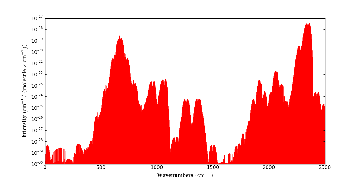
Carbon dioxide line intensities between 0 and 2500 wavenumbers (HITRAN2012)

I can also calculate the Planck (blackbody) shape for 255 K, the effective radiation temperature of the Earth:

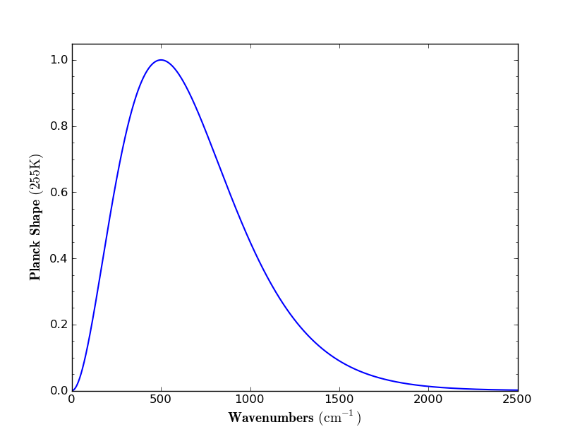
Planck shape (blackbody) for 255 K

and see the effect of scaling the line strengths by the blackbody shape, convoluting line-strength with amount of energy.

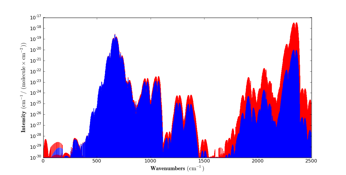
Carbon dioxide line intensities from 0 to 2500 wavenumbers (HITRAN2012). Unweighted intensities are in red. Intensities weighted by the Planck (blackbody) shape for 255 K are shown in blue.

One of the rules of thumb is that radiation can escape to space from the altitude at which the optical path from the top of the atmosphere is about one, including a diffusivity factor to account for the radiation traveling at different angles relative to the vertical. That diffusivity factor is often taken to be 1.66, corresponding to an average angle of about 53 degrees. Using that rule of thumb, I’ve estimated the corresponding altitudes for 300 ppm of CO₂ (blue) and 600  of CO₂ (red). I’ve added a black line representing the tropical tropopause. Any red seen below that line represents emission moved to a colder temperature due to doubling CO₂. Since a colder temperature radiates less energy, there’s the basis for the CO₂ greenhouse forcing.

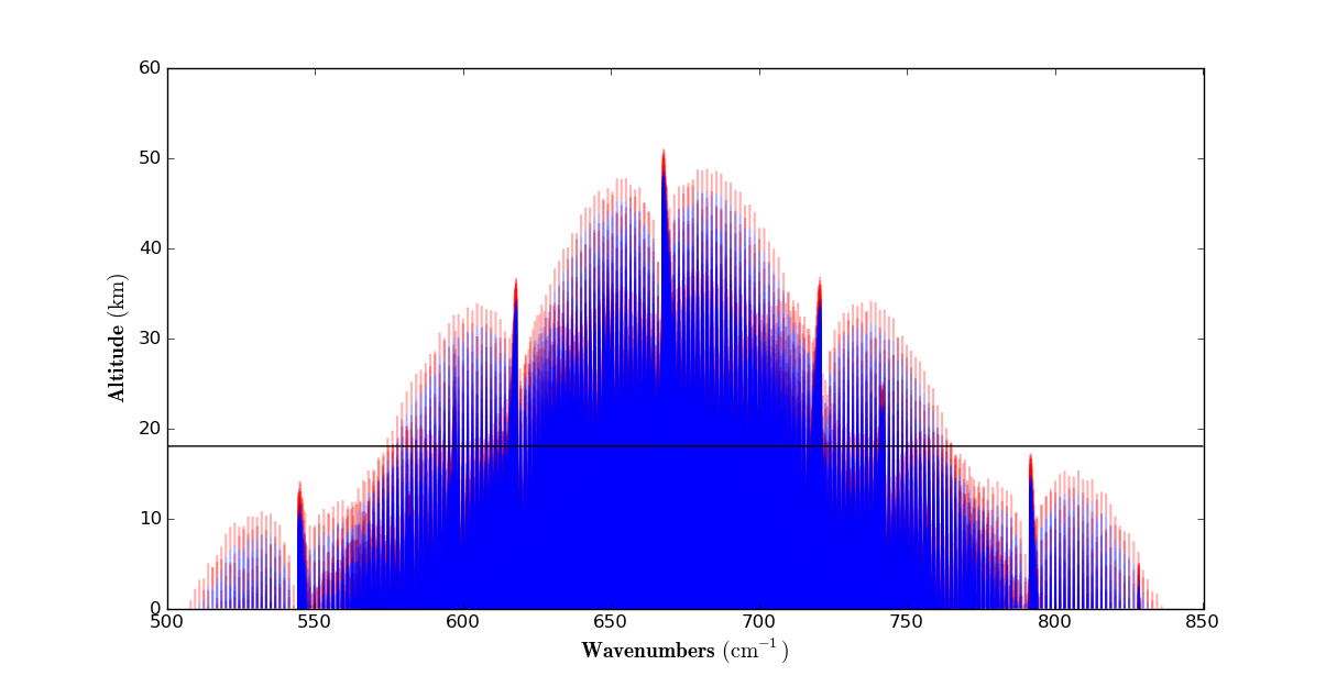
Approximate altitudes at which the carbon dioxide optical paths from space as a function of wavenumber are one. Shown in blue for 300 ppm CO₂ and red for 600 ppm. Linear pressure scaling and a diffusivity factor of 1.66 were included. Lines integrated with a Lorenz shape, increment of 0.01 cm^-1, and cutoff of 20 cm^-1.

Andy Dessler also hits this part of physics in his recent video How the greenhouse effect works

One final area I wanted to touch on in this post is the amount of effort the Air Force put into understanding the atmosphere and atmospheric radiative transfer. I’ve already added a quote above to this effect with HITRAN. An interview with Larry Rothman adds to that history as does the sequence of spectroscopic reports dating back to 1973. Bob McClatchey et al. put out a series of atmospheric profiles that became standards for testing and comparing radiative transfer models. In 1985, the Air Force Geophysics Laboratory published the 4th edition of their Handbook of Geophysics and Space Environments. Chapter 18, in particular, dealt with atmospheric radiative transfer.

Many of the people involved with these efforts continued on with them. Larry Rothman with HITRAN, Gail Anderson with the LowTran and ModTran models. Tony Clough at AER working on the water vapor continuum and RRTM models, Eric Shettle with characterization and satellite retrievals of atmospheric aerosols. I can’t emphasize too much the amount of history and effort behind all of this nor the solidity and pragmatism of those who helped bring us to where we are today. The forward radiative transfer models, spectroscopic data and algorithms, also are an essential part of retrieving physical measurements from both civilian and military satellite observations; observations which have been subjected to many comparisons and in situ verifications.